Classification Analysis

Classification analysis assigns an observation to a group based on its measured variables, using patterns from known group data.

Imagine sorting fruit into baskets: you measure features (e.g., weight, color), compare them to known apples and oranges, and pick the closest match.

A new observation vector $\mathbf{y}$ is compared to previous observartions to predict its group, often via a discriminant score.

Purpose of classification

Classification predicts group membership for unknown observations, using prior samples. It’s valuable for:

• Prediction (e.g., student success, mental illness category).
• Decision-making (e.g., identifying “killer” bees).
• Allocation (e.g., matching trainees to programs).

Unlike discriminant analysis, it focuses on allocation, not just separation.

Classification procedures

• Classifying Observations into Two Groups
• Classifying Observations into Several Groups
• Nonparametric Classification Procedures

Estimating misclassification rates

1. Use training data to define the classification rule.

2. Apply the rule to every observation ${\mathbf{y}}_{ij}$ in the training set to predict its group.

3. For each ${\mathbf{y}}_{ij}$, check if the predicted group matches its actual group.

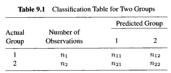
4. Count Misclassifications: Use a classification table (such as Table 9.1)

   For 2 groups:

   • $n_{11}$: Correctly classified into $G_1$
   • $n_{12}$: Misclassified into $G_2$
   • $n_{21}$: Misclassified into $G_1$
   • $n_{22}$: Correctly classified into $G_2$.

   For $k$ groups, sum all off-diagonal counts in the classification table (e.g., $n_{12}+n_{13}+n_{21}+\cdots$).

5. Compute Rate (Formula 9.16):

   \text{Apparent Error Rate} &= \frac{\text{Total Misclassifications}}{\text{Total Observations}}\\ &= \frac{n_{12} + n_{21}}{n_{1} + n_{2}}\\ &= \frac{n_{12} + n_{21}}{n_{11} + n_{12} + n_{21} + n_{22}}\\ \end{align}$$

Classification table example:

Python example

For classification into two groups, see example on Python example

The example below demonstrates 2 classifications into 3 groups, one assuming equal covariance, the other assuming unequal covariance.

import numpy as np
 
# Football data means (Example 9.3.1, 6 variables simplified to 2 for brevity)
y_bar_1 = np.array([15.2, 58.9])  # Group 1
y_bar_2 = np.array([15.4, 57.4])  # Group 2
y_bar_3 = np.array([15.6, 57.8])  # Group 3
means = [y_bar_1, y_bar_2, y_bar_3]
 
# Simplified covariance matrices
S_pl = np.array([[2.5, 0.8], [0.8, 3.0]])  # Pooled (equal covariance)
S_1 = np.array([[2.0, 0.5], [0.5, 2.5]])   # Group 1
S_2 = np.array([[2.8, 0.9], [0.9, 3.2]])   # Group 2
S_3 = np.array([[2.2, 0.7], [0.7, 2.8]])   # Group 3
covs = [S_1, S_2, S_3]
 
# New observation (first in Group 1)
y_new = np.array([13.5, 57.2])
 
# Equal Covariance (Formula 9.11)
S_pl_inv = np.linalg.inv(S_pl)
L = []
for i, y_bar in enumerate(means):
    term1 = y_bar @ S_pl_inv @ y_new
    term2 = 0.5 * y_bar @ S_pl_inv @ y_bar
    L_i = term1 - term2  # L_i(y)
    L.append(L_i)
group_linear = np.argmax(L) + 1
 
# Unequal Covariance (Formula 9.15, assume equal priors p_i = 1/3)
Q = []
for i, (y_bar, S_i) in enumerate(zip(means, covs)):
    S_i_inv = np.linalg.inv(S_i)
    diff = y_new - y_bar
    term1 = np.log(1/3)  # ln p_i
    term2 = 0.5 * np.log(np.linalg.det(S_i))
    term3 = 0.5 * diff @ S_i_inv @ diff
    Q_i = term1 - term2 - term3  # Q_i(y)
    Q.append(Q_i)
group_quadratic = np.argmax(Q) + 1
 
print("Linear scores:", list(map(int, L)))
print("Predicted group (linear):", group_linear)
print("Quadratic scores:", list(map(int, Q)))
print("Predicted group (quadratic):", group_quadratic)

Linear scores: [545, 545, 545]
Predicted group (linear): 2
Quadratic scores: [-2, -2, -2]
Predicted group (quadratic): 2