Nonparametric Classification Procedures

When data deviates from normality, nonparametric methods classify observations without assuming a specific distribution.

This note will describe 4 nonparametric classification procecures.

Each uses sample data directly to assign ${\mathbf{y}}_0$ to one of $k$ groups.

Multinomial classification

Treats variables as categorical (e.g., counts or discrete levels), comparing observed frequencies to expected ones per group.

For an observation $\mathbf{y}$ with frequency $q_{hi}$ in group $G_h$:

• Assign to $G_1$ if $\frac{q_{1i}}{q_{2i}}>\frac{p_2}{p_1}$ (Formula 9.17, two groups), else $G_2$.
• For $k>2$, assign to group $h$ maximizing $p_h{q}_{hi}$ (generalized rule).

Steps:

1. Categorize Data: Convert continuous $\mathbf{y}$ into discrete levels (e.g., bins) or use naturally categorical data.
2. Count Frequencies: For each category $i$ in $\mathbf{y}$, count occurrences $q_{hi}$ in training data for group $G_h$.
3. Estimate Priors: Set prior probability $p_h$ (e.g., $p_h=n_h/N$ or equal if unspecified).
4. Compute Ratios (2 Groups): For each category $i$, calculate $\frac{q_{1i}}{q_{2i}}$ and compare to $\frac{p_2}{p_1}$.
5. Classify: If ratio > threshold, assign to $G_1$; else $G_2$. For $k>2$, compute $p_h{q}_{hi}$ for all $h$ and pick max.

Classification based on density estimators

Estimates the probability density $f_h(\mathbf{y})$ for each group using a kernel (e.g., normal) and assigns $\mathbf{y}$ to the group with the highest density.

Steps

1. Compute kernel density estimate (9.23):

   $$\hat{f}({\mathbf{y}}_0)=\frac{1}{n{h}_1{h}_2\dots h_p}\sum _{i=1}^{n}K\left(\frac{y_{01}-y_{i1}}{h_1},\dots ,\frac{y_{0p}-y_{ip}}{h_p}\right)$$

   where

   • $K(u)$: Kernel (e.g., normal)
   • $h$: Smoothing parameter (e.g., $h=2$ from Table 9.8)
   • $p$: Amount of variables
   • $n$: Sample size

2. Assign to group $h$ which has the maximum $p_i\hat{f}({\mathbf{y}}_0|G_i)$ (9.28), where $p_i$ is the $i$-th prior probability.

Nearest neighbor classificaton rule

Assigns ${\mathbf{y}}_i$ to the group most common among its $k$ closest observations, based on distance.

Steps:

1. Compute distances of ${\mathbf{y}}_i$ to other points using the distance function:

   $$({\mathbf{y}}_i-{\mathbf{y}}_j{)}^{\prime }{\mathbf{S}}_{pl}^{-1}({\mathbf{y}}_i-{\mathbf{y}}_j),i\ne j$$

2. Assign to group with highest count among $k$ nearest neighbors. For 2 groups, assign ${\mathbf{y}}_i$ to $G_1$ if:

   $$\frac{k_1}{n_1}>\frac{k_2}{n_2}$$

   Or for further refinement, use prior probabilities:

   $$\frac{k_1/n_1}{k_2/n_2}>\frac{p_2}{p_1}$$

   For $i$ groups, assign the observation to the group that has the highest $\frac{k_i}{n_i}$ Where:

   • $k_i$ number of observations from $G_i$ among the $k$ nearest neighbors of the observation in question.

We suggest choosing $k$ nearing $\sqrt{n_i}$.

In practice, one could test several values of $k$, and use one with the best error rate.

When data deviates from normality, nonparametric methods classify observations without assuming a specific distribution.

This note will describe 4 nonparametric classification procecures.

Each uses sample data directly to assign ${\mathbf{y}}_0$ to one of $k$ groups.

Multinomial classification

Treats variables as categorical (e.g., counts or discrete levels), comparing observed frequencies to expected ones per group.

For an observation $\mathbf{y}$ with frequency $q_{hi}$ in group $G_h$:

• Assign to $G_1$ if $\frac{q_{1i}}{q_{2i}}>\frac{p_2}{p_1}$ (Formula 9.17, two groups), else $G_2$.
• For $k>2$, assign to group $h$ maximizing $p_h{q}_{hi}$ (generalized rule).

Steps:

1. Categorize Data: Convert continuous $\mathbf{y}$ into discrete levels (e.g., bins) or use naturally categorical data.
2. Count Frequencies: For each category $i$ in $\mathbf{y}$, count occurrences $q_{hi}$ in training data for group $G_h$.
3. Estimate Priors: Set prior probability $p_h$ (e.g., $p_h=n_h/N$ or equal if unspecified).
4. Compute Ratios (2 Groups): For each category $i$, calculate $\frac{q_{1i}}{q_{2i}}$ and compare to $\frac{p_2}{p_1}$.
5. Classify: If ratio > threshold, assign to $G_1$; else $G_2$. For $k>2$, compute $p_h{q}_{hi}$ for all $h$ and pick max.

Classification based on density estimators

Estimates the probability density $f_h(\mathbf{y})$ for each group using a kernel (e.g., normal) and assigns $\mathbf{y}$ to the group with the highest density.

Steps

1. Compute kernel density estimate (9.23):

   $$\hat{f}({\mathbf{y}}_0)=\frac{1}{n{h}_1{h}_2\dots h_p}\sum _{i=1}^{n}K\left(\frac{y_{01}-y_{i1}}{h_1},\dots ,\frac{y_{0p}-y_{ip}}{h_p}\right)$$

   where

   • $K(u)$: Kernel (e.g., normal)
   • $h$: Smoothing parameter (e.g., $h=2$ from Table 9.8)
   • $p$: Amount of variables
   • $n$: Sample size

2. Assign to group $h$ which has the maximum $p_i\hat{f}({\mathbf{y}}_0|G_i)$ (9.28), where $p_i$ is the $i$-th prior probability.

Nearest neighbor classificaton rule

Assigns ${\mathbf{y}}_i$ to the group most common among its $k$ closest observations, based on distance.

Steps:

1. Compute distances of ${\mathbf{y}}_i$ to other points using the distance function:

   $$({\mathbf{y}}_i-{\mathbf{y}}_j{)}^{\prime }{\mathbf{S}}_{pl}^{-1}({\mathbf{y}}_i-{\mathbf{y}}_j),i\ne j$$

2. Assign to group with highest count among $k$ nearest neighbors. For 2 groups, assign ${\mathbf{y}}_i$ to $G_1$ if:

   $$\frac{k_1}{n_1}>\frac{k_2}{n_2}$$

   Or for further refinement, use prior probabilities:

   $$\frac{k_1/n_1}{k_2/n_2}>\frac{p_2}{p_1}$$

   For $i$ groups, assign the observation to the group that has the highest $\frac{k_i}{n_i}$ Where:

   • $k_i$ number of observations from $G_i$ among the $k$ nearest neighbors of the observation in question.

We suggest choosing $k$ nearing $\sqrt{n_i}$.

In practice, one could test several values of $k$, and use one with the best error rate.

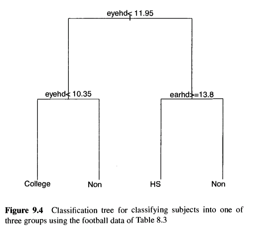
Classification Trees

Builds a decision tree by recursively splitting data into nodes based on predictor variables, assigning ${\mathbf{y}}_0$ to the group most common in its terminal node.

Steps:

1. Start at root node: Place all $n$ observations (training data) in one group (root node).

2. Choose split: For each predictor variable $x_j$, test all possible cutoffs to split the node into two child nodes ($A_L$ and $A_R$):

   • Compute impurity $I_A={\sum }_{i=1}^k{p}_{i|A}(1-p_{i|A})$ (Gini index, 9.32) for the parent node $A$, where $p_{i|A}=\frac{p_i(n_{iA}/n_i)}{{\sum }_{i=1}^k{p}_i(n_{iA}/n_i)}$ (9.35).
   • Compute impurity for child nodes $I_{A_L}$ and $I_{A_R}$.
   • Calculate change in impurity: $\Delta I=p_A{I}_A-(p_{A_L}{I}_{A_L}+p_{A_R}{I}_{A_R})$ (9.36), where $p_A=\frac{n_A}{n}$.
   • Select the variable and cutoff maximizing $\Delta I$ (best split).

3. Repeat recursively: Apply step 2 to each child node (e.g., $A_L$, $A_R$) until a stopping rule (e.g., cross-validation) determines the optimal tree size. Nodes that stop splitting are terminal nodes.

4. Assign groups: For each terminal node, assign the group $G_i$ with the highest count.

5. Classify ${\mathbf{y}}_0$: Traverse the tree with ${\mathbf{y}}_0$‘s values:

   • Start at the root, follow splits (e.g., if eyehd < 11.95, go left).
   • Reach a terminal node and assign ${\mathbf{y}}_0$ to its group.

Python example

import numpy as np
from scipy.stats import multivariate_normal
 
# Simplified football data (3 groups, 2 variables: e.g., speed, strength)
G1 = np.array([[15.2, 58.9], [14.8, 59.1], [15.0, 58.7], [15.4, 59.0], [14.9, 58.8]])
G2 = np.array([[15.4, 57.4], [15.6, 57.2], [15.3, 57.6], [15.5, 57.3], [15.2, 57.5]])
G3 = np.array([[15.6, 57.8], [15.8, 57.6], [15.7, 57.9], [15.5, 57.7], [15.9, 57.8]])
X = np.vstack([G1, G2, G3])  # All training data
y = np.array([1]*5 + [2]*5 + [3]*5)  # Labels: 1, 2, 3
n_groups = 3
n_per_group = 5
new_y = np.array([13.5, 57.2])  # New observation
 
# --- Multinomial Classification ---
# Bin into 3 categories per variable (low, med, high)
bins = [np.percentile(X[:, i], [0, 33, 66, 100]) for i in range(2)]
y_cat = [np.searchsorted(bins[i][1:-1], new_y[i], side='right') for i in range(2)]
X_cat = np.array([np.searchsorted(bins[i][1:-1], X[:, i], side='right') for i in range(2)]).T
cat_idx = X_cat[:, 0] * 3 + X_cat[:, 1]  # Index for 2D categories
new_idx = y_cat[0] * 3 + y_cat[1]
 
# Counts for each group in the new category (with small smoothing to avoid zeros)
q_hi = [np.sum((cat_idx == new_idx) & (y == h)) + 0.01 for h in range(1, 4)]
p_h = [1/3] * 3  # Equal priors
scores_multinomial = [p_h[i] * q_hi[i] for i in range(3)]
group_multinomial = np.argmax(scores_multinomial) + 1
 
# --- Density Estimation ---
h = 2.0  # Bandwidth from Table 9.8
p = 2  # Dimensions
kernel_const = (2 * np.pi)**(-p/2)  # Normal kernel constant
f_h = []
for h_idx in range(n_groups):
    group_data = X[h_idx * n_per_group:(h_idx + 1) * n_per_group]
    kernel_sum = 0
    for x in group_data:
        u = (new_y - x) / h
        kernel_sum += kernel_const * np.exp(-0.5 * np.sum(u**2))
    density = kernel_sum / (n_per_group * h**p)
    f_h.append(density)
scores_density = [p_h[i] * f_h[i] for i in range(n_groups)]
group_density = np.argmax(scores_density) + 1
 
# --- Nearest Neighbor (k=5) ---
distances = np.sqrt(np.sum((X - new_y)**2, axis=1))  # Euclidean distance
k = 5
nearest_idx = np.argsort(distances)[:k]  # Indices of k smallest distances
nearest_labels = y[nearest_idx]
counts = np.zeros(n_groups + 1, dtype=int)  # Manual bincount
for label in nearest_labels:
    counts[label] += 1
group_nn = np.argmax(counts[1:]) + 1  # Ignore index 0
 
# --- Classification Tree ---
# Fixed tree with proper branching
def classify_tree(x, X, y):
    if x[0] < 15.5:  # First split
        if x[1] < 58.0:  # Second split for left branch
            region = (X[:, 0] < 15.5) & (X[:, 1] < 58.0)
        else:
            region = (X[:, 0] < 15.5) & (X[:, 1] >= 58.0)
    else:  # Right branch of first split
        if x[1] < 58.0:  # Second split for right branch
            region = (X[:, 0] >= 15.5) & (X[:, 1] < 58.0)
        else:
            region = (X[:, 0] >= 15.5) & (X[:, 1] >= 58.0)
    
    region_labels = y[region]
    if len(region_labels) == 0:  # Default to most common group
        return np.argmax(np.bincount(y)[1:]) + 1
    
    group_counts = np.bincount(region_labels, minlength=n_groups+1)
    return np.argmax(group_counts[1:]) + 1
 
group_tree = classify_tree(new_y, X, y)
 
# Results - format as floats to preserve small values
print("Multinomial scores:", [f"{score:.6e}" for score in scores_multinomial])
print("Predicted group (multinomial):", group_multinomial)
print("Density scores:", [f"{score:.6e}" for score in scores_density])
print("Predicted group (density):", group_density)
print("Nearest neighbor counts for groups 1,2,3 (k=5):", counts[1:])
print("Predicted group (nearest neighbor):", group_nn)
print("Predicted group (tree):", group_tree)

Multinomial scores: ['3.333333e-03', '3.366667e-01', '3.333333e-03']
Predicted group (multinomial): 2
Density scores: ['6.801202e-03', '8.378014e-03', '6.959560e-03']
Predicted group (density): 2
Nearest neighbor counts for groups 1,2,3 (k=5): [0 4 1]
Predicted group (nearest neighbor): 2
Predicted group (tree): 2