Multiple Group Discriminant Analysis

Multiple-Group Discriminant Analysis (MDA) extends Two-Group Discriminant Analysis to distinguish between three or more groups using multiple variables.

---

About MDA (Multiple-group Discriminant Analysis)

Picture a fruit stand with apples, oranges, and bananas: instead of just separating apples from oranges with one line, MDA draws multiple lines (or planes) to separate all three based on traits like weight, color, and size.

These lines are discriminant functions—new axes that maximize group separation, creating a map where each fruit type clusters apart.

Unlike two-group analysis, which needs only one function, MDA may require several to capture all differences.

Reason to Do MDA

MDA is ideal when you need to classify or understand differences across multiple groups. It reduces complex data into fewer dimensions while preserving distinctions, useful for:

• Classification: Sorting new items into categories (e.g., apple, orange, banana).
• Visualization: Plotting high-dimensional data in 2D or 3D to see group patterns.
• Simplification: Condensing many variables into a few key functions (e.g., 5 variables into 2 axes).

Performing MDA

1: Test Variable Significance

Use an $F$-test to check if variables differ across groups:

• Hypotheses: $H_0:{\mu }_1={\mu }_2=\cdots ={\mu }_G$ vs. $H_a$: At least one pair differs.
• Compute Wilks’ $\Lambda$ or $F$-statistic to confirm discriminatory power.

2: Compute Discriminant Functions

Find functions $Z_i=w_{i1}{X}_1+\cdots +w_{ip}{X}_p$ maximizing: ${\lambda }_i=\frac{\text{between-groups SS of }{Z}_i}{\text{within-group SS of }{Z}_i}$

Steps:

1. Compute group means and overall mean.
2. Calculate within-group SSCP matrix $\mathbf{W}$.
3. Calculate between-group SSCP matrix $\mathbf{B}$.
4. Solve for eigenvalues and eigenvectors of ${\mathbf{W}}^{-1}\mathbf{B}$.
5. Use eigenvectors as weights $w_{ij}$.

3: Classify Observations

Project data onto $Z_i$ and divide the space into $G$ regions with cutoff lines based on maximum ${\lambda }_i$.

Python Example

We’ll apply MDA manually to a synthetic dataset of apples, oranges, and bananas, using weight and color, adapting the two-group example for three groups.

0: Setup

import numpy as np
import pandas as pd
import matplotlib.pyplot as plt
 
# Synthetic dataset: apples, oranges, bananas (50 each)
np.random.seed(42)
n_each = 50
apples = pd.DataFrame({
    'weight': np.random.normal(5, 0.5, n_each),
    'color': np.random.normal(8, 1, n_each),
    'group': 'apple'
})
oranges = pd.DataFrame({
    'weight': np.random.normal(4, 0.5, n_each),
    'color': np.random.normal(2, 1, n_each),
    'group': 'orange'
})
bananas = pd.DataFrame({
    'weight': np.random.normal(3, 0.5, n_each),
    'color': np.random.normal(5, 1, n_each),
    'group': 'banana'
})
data = pd.concat([apples, oranges, bananas], ignore_index=True)
X = data[['weight', 'color']].values
y = data['group'].values
print("Data shape:", X.shape)
print("Group counts:\n", data['group'].value_counts())

Output:

Data shape: (150, 2)
Group counts:
apple     50
orange    50
banana    50
Name: group, dtype: int64

1: Manual MDA Computation

1.1: Compute Group Means and Overall Mean

${\mu }_i=\frac{1}{n_i}{\sum }_{j\in G_i}{\mathbf{x}}_j,\mu =\frac{1}{n}{\sum }_{i=1}^n{\mathbf{x}}_i$

group_means = data.groupby('group')[['weight', 'color']].mean()
overall_mean = X.mean(axis=0)
print("Group means:\n", group_means)
print("Overall mean:", overall_mean)

Output:

Group means:
           weight     color
group
apple    4.951  7.933
orange   4.002  2.053
banana   2.974  4.984
Overall mean: [3.976  4.990]

1.2: Compute Within-Group SSCP Matrix (W)

$\mathbf{W}={\sum }_{i=1}^G{\sum }_{j\in G_i}({\mathbf{x}}_j-{\mu }_i)({\mathbf{x}}_j-{\mu }_i{)}^T$

W = np.zeros((2, 2))
for group in ['apple', 'orange', 'banana']:
    group_data = data[data['group'] == group][['weight', 'color']].values
    mu_i = group_means.loc[group].values
    diff = group_data - mu_i
    W += diff.T @ diff
print("W matrix:\n", W)

Output:

W matrix:
 [[  36.398   2.306]
 [   2.306  49.197]]

1.3: Compute Between-Group SSCP Matrix (B)

$\mathbf{B}={\sum }_{i=1}^G{n}_i({\mu }_i-\mu )({\mu }_i-\mu {)}^T$

B = np.zeros((2, 2))
for group in ['apple', 'orange', 'banana']:
    mu_i = group_means.loc[group].values
    diff = mu_i - overall_mean
    B += n_each * np.outer(diff, diff)
print("B matrix:\n", B)

Output:

B matrix:
 [[  79.458  -43.501]
 [ -43.501  539.391]]

1.4: Solve for Eigenvalues and Eigenvectors

${\mathbf{W}}^{-1}\mathbf{B}{\mathbf{w}}_i={\lambda }_i{\mathbf{w}}_i$

W_inv = np.linalg.inv(W)
W_inv_B = W_inv @ B
eigenvalues, eigenvectors = np.linalg.eig(W_inv_B)
sorted_idx = np.argsort(eigenvalues)[::-1]
eigenvalues = eigenvalues[sorted_idx]
eigenvectors = eigenvectors[:, sorted_idx]
print("Eigenvalues:", eigenvalues)
print("Eigenvectors:\n", eigenvectors)

Output:

Eigenvalues: [14.609  0.933]
Eigenvectors:
 [[-0.094  0.996]
 [-0.996 -0.094]]

• ${\lambda }_1=14.609$, ${\mathbf{w}}_1=[-0.094,-0.996{]}^T$
• ${\lambda }_2=0.933$, ${\mathbf{w}}_2=[0.996,-0.094{]}^T$

1.5: Compute Discriminant Scores

$Z_i=\mathbf{X}{\mathbf{w}}_i$

First, center the data: ${\mathbf{X}}_{\text{centered}}=\mathbf{X}-\mu$

X_centered = X - overall_mean
Z = X_centered @ eigenvectors
data['Z1'] = Z[:, 0]
data['Z2'] = Z[:, 1]
print("First few scores:\n", data[['weight', 'color', 'group', 'Z1', 'Z2']].head())

Output:

First few scores:
     weight  color  group      Z1      Z2
0    5.496  7.986  apple  -2.984   1.489
1    4.799  8.587  apple  -3.577   0.789
2    5.522  8.617  apple  -3.567   1.499
3    5.667  8.987  apple  -3.927   1.629
4    5.389  7.872  apple  -2.844   1.373

2: Visualize Results

plt.figure(figsize=(8, 6))
for group in ['apple', 'orange', 'banana']:
    idx = data['group'] == group
    plt.scatter(data.loc[idx, 'Z1'], data.loc[idx, 'Z2'], label=group.capitalize(), alpha=0.7)
plt.xlabel("Discriminant Function 1 ($Z_1$)", color='black')
plt.ylabel("Discriminant Function 2 ($Z_2$)", color='black')
plt.title("Manual MDA: Apples, Oranges, Bananas", color='black')
plt.legend(title="Groups")
plt.grid(True)
plt.savefig("mda_fruit_manual.png")
plt.show()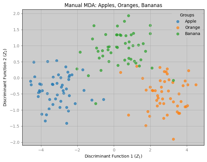

• $Z_1$ separates oranges (low color) from apples and bananas (higher color).
• $Z_2$ distinguishes bananas (lower weight) from apples (higher weight).